POMDPy

This open-source project contains a framework for implementing discrete action/state POMDPs in Python.
Here’s David Silver and Joel Veness’s paper on POMCP, a ground-breaking POMDP solver. Monte-Carlo Planning in Large POMDPs
This project has been conducted strictly for research purposes.
If you use this work in your research, please cite with:
@ARTICLE{emami2015pomdpy,
  author = {Emami, Patrick and Hamlet, Alan J., and Crane, Carl},
  title = {POMDPy: An Extensible Framework for Implementing POMDPs in Python},
  year = {2015},
}
Dependencies
Download the files as a zip or clone into the repository.
git clone https://github.com/pemami4911/POMDPy.git
This project uses:
- numpy >= 1.11
- matplotlib >= 1.4.3
- scipy >= 0.15.1
- future >= 0.16
- tensorflow >= 0.12
See the Tensorflow docs for information about installing Tensorflow.
The easiest way to satisfy the dependencies is to use Anaconda. You might have to run pip install --upgrade future after installing Anaconda, however.
Supported Solvers
POMCP
POMCP uses the off-policy Q-Learning algorithm and the UCT action-selection strategy. It is an anytime planner that approximates the action-value estimates of the current belief via Monte-Carlo simulations before taking a step. This is known as Monte-Carlo Tree Search (MCTS).
To solve a POMDP with POMCP, the following classes should be implemented:
- Discrete Action
- Discrete State
- Discrete Observation
- Discrete/Enumerated ActionPool
-
Model - this module is the most important, since it acts as the black-box generator for (S’, A, O, R) steps. This also encodes the belief update rule for the particle filter.
You may want to to provide a .txt of .cfg containing a map or other data that encapsulate the environment and hence the transition probabilities for the world which the POMDP lives in.
Heirarchy of nodes in the belief tree from a parent BeliefNode to a child BeliefNode:
(parent) BeliefNode -> ActionMapping -> ActionMappingEntry -> ActionNode -> ObservationMap -> ObservationMappingEntry -> (child) BeliefNode
Value Iteration
Implemented with Lark’s pruning algorithm.
Running an example
You can run tests with POMCP on RockSample, and use Value Iteration to solve the Tiger example.
Note: The RockSample env needs some work to fully match up with the implementation described in Silver et al.
You can optionally edit the RockSample configuration file rock_sample_config.json to change the map size or environment parameters.
This file is located in pompdy/config.
The following maps are available:
- RockSample(7, 8), a 7 x 7 grid with 8 rocks.
- RockSample(11, 11), an 11 x 11 grid with 11 rocks
- RockSample(15, 15), a 15 x 15 grid with 15 rocks
- As well as a few others, such as (7, 2), (7, 3), (12, 12), and more. It is fairly easy to make new maps.
To run RockSample with POMCP:
python pomcp.py --env RockSample --solver POMCP --max_steps 200 --epsilon_start 1.0 --epsilon_decay 0.99 --n_epochs 10 --n_sims 500 --preferred_actions --seed 123
To run the Tiger example with the full-width planning value iteration algorithm:
python vi.py --env Tiger --solver ValueIteration --planning_horizon 8 --n_epochs 10 --max_steps 10 --seed 123
To run the Tiger example with linear value function approximation:
python vi.py --env Tiger --solver LinearAlphaNet --use_tf --n_epochs 5000 --max_steps 50 --test 5 --learning_rate 0.05 --learning_rate_decay 0.996 --learning_rate_minimum 0.00025 --learning_rate_decay_step 50 --beta 0.001 --epsilon_start 0.2 --epsilon_minimum 0.02 --epsilon_decay 0.99 --epsilon_decay_step 75 --seed 12157 --save
Experiment Notes
To determine whether it is possible to approximate a value function for a small POMDP, I used simple linear function approximation to predict the pruned set of alpha vectors. For the Tiger problem, one can visually inspect the value function with a planning horizon of eight, and see that it can be approximated by three well-placed alpha vectors. Using the one-step rewards for each of the three actions as a basis function, I designed a linear approximation to the value function .
Each alpha vector has the same dimension as the belief state space. I initialized all weights to 1.0, so that
the agent essentially started learning from a planning horizon of 1 (greedy action-selection with no planning).
The goal of this learning task is to determine whether the classic value iteration algorithm having exponential run time complexity can be avoided with function approximation. For baselines, I compared against planning horizons of one and eight, computed with Lark’s pruning algorithm, as well as a random agent.
Baseline Results
Results averaged over 5 experiments with different random seeds
| planning horizon | epochs/experiment | mean reward/epoch | std dev reward/epoch | mean wrong door count |
|---|---|---|---|---|
| 8 | 1000 | 4.703091980822256 | 8.3286422581 | 102.4 |
| 1 | 1000 | 4.45726700400672 | 10.3950449814 | 148.6 |
| random | 1000 | -5.466722724994926 | 14.6177021188 | 503.0 |
The mean wrong door counts represent the number of times the agent opened the door with the tiger.
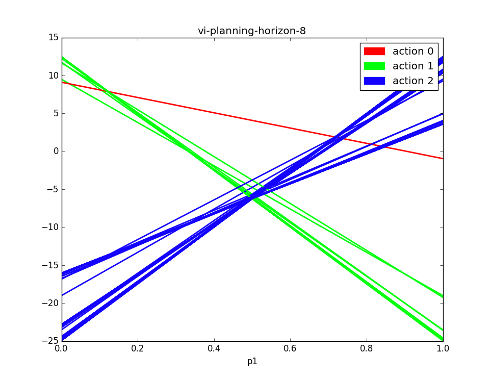
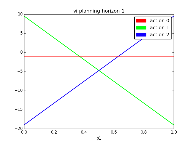
Here are plots of the alpha vectors returned by the classic value iteration algorithm.
There are 77 alpha vectors in the value function for the planning horizon of 8.


Linear Function Approximation
The best results so far were obtained with the following parameters:
{'beta': 0.001,
 'discount': 0.95,
 'env': 'Tiger',
 'epsilon_decay': 0.99,
 'epsilon_decay_step': 75,
 'epsilon_minimum': 0.02,
 'epsilon_start': 0.2,
 'learning_rate': 0.05,
 'learning_rate_decay': 0.996,
 'learning_rate_decay_step': 50,
 'learning_rate_minimum': 0.00025,
 'max_steps': 50,
 'n_epochs': 5000,
 'planning_horizon': 5,
 'save': True,
 'seed': 12157,
 'solver': 'LinearAlphaNet',
 'test': 5,
 'use_tf': True}
After doing a hyperparameter search, the learning rate of 0.05 was chosen with an exponential decay of 0.996 every 50
steps, until the learning rate is at 0.00025. The Momentum optimizer is used with a parameter of 0.8. L2 regularization
with a beta parameter of 0.001 is chosen via a parameter search as well.
To encourage exploration, e-greedy action-selection is added. This way, early on during training, the agent isn’t overly
greedy given that the weights are initialized to 1.0 to simulate a planning horizon of 1.
Training is carried out by running for 5000 epochs, where each epoch consisted of 50 agent interactions with the environment.
The agent is evaluated every 5 epochs to test its progress.
Results
After training, the agent is tested by averaging 5 runs with different random seeds, where each run consists of 1000 epochs.
| epochs/experiment | mean reward/epoch | std dev reward/epoch | mean wrong door count |
|---|---|---|---|
| 1000 | 4.286225210218933 | 10.0488961427 | 145.8 |
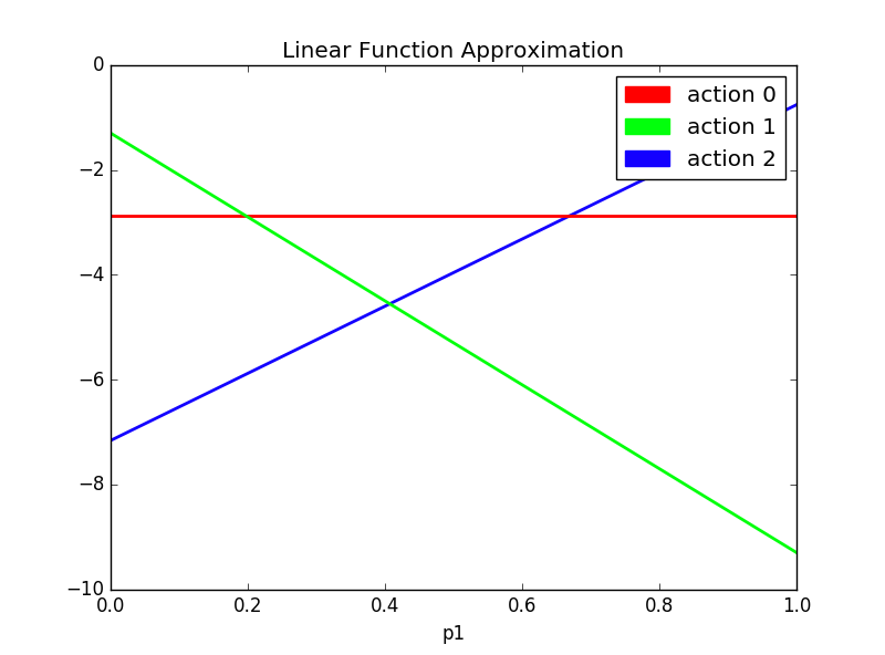
 This figure depicts the alpha vectors as computed after training the linear function approximator.
There is not a statistically significant improvement over the performance of a planning horizon of 1.
Some reasons for this are:
-
The objective function is minimizing the MSE of the predicted value function for a given belief and the predicted value function for the transformed belief given the current action and observation. This objective function doesn’t encourage the agent to do things like explore actions that are more informative than others. In fact, the agent is quite happy to find some nearby local minima that allows its value function to be “self-consistent”, i.e., it looks like the agent has converged onto the optimal value function, but in fact it has found a biased solution. This is a common problem found with objective functions modeled after Temporal Difference Learning.
-
This learning approach is highly sensitive to the number of alpha vectors and their initialization. In this case, I can visually inspect the value function with a planning horizon of
8and see that3vectors suffice. Hence, I am satisfied to initialize my3approximate alpha-vectors to be the immediate rewards gleaned from the3actions.
One suggested improvement is adding an auxiliary task to the agent’s loss function that seeks to maximize its information gain about the effects of its actions on the environment.
Another suggestion is to implement experience replay and target networks, to force the agent to train more slowly and to de-correlate its experiences.
The agent needs to learn that listening more than once allows it to successfully open the correct door with a higher probability. This is difficult, because listening has a slight negative reward, so that a sequence of actions consisting of listening once or twice followed by opening the correct door has a lower discounted reward than simply guessing the correct door without listening at all. This implies that the objective function for the RL agent should be maximizing expected discounted return over multiple trajectories. This suggests that the use of mini-batches and experience replay could also improve performance.
Approximating the piece-wise linear and convex value function with a smooth, nonlinear function is also of interest. This was done by Parr and Russell with SPOVA, but SPOVA was also plagued by needing good initializations, uncertain number of alpha vectors to approximate, and uses the TD-learning objective function. A simple MLP could potentially be used as well.
