Deep Deterministic Policy Gradients in TensorFlow
By: Patrick Emami
Introduction
Deep Reinforcement Learning has recently gained a lot of traction in the machine learning community due to the significant amount of progress that has been made in the past few years. Traditionally, reinforcement learning algorithms were constrained to tiny, discretized grid worlds, which seriously inhibited them from gaining credibility as being viable machine learning tools. Here’s a classic example from Richard Sutton’s book, which I will be referencing a lot.
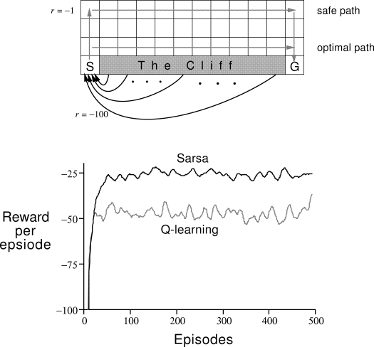
Cliff-walking task, Fig. 6.4 from [1]
After Deep Q-Networks [3] became a hit, people realized that deep learning methods could be used to solve high-dimensional problems. One of the subsequent challenges that the reinforcement learning community faced was figuring out how to deal with continuous action spaces. This is a significant obstacle, since most interesting problems in robotic control, etc., fall into this category. Logically, if you discretize your continuous action space too finely, you end up with the same curse of dimensionality problem as before. On the other hand, a naive discretization of the action space throws away valuable information concerning the geometry of the action domain.
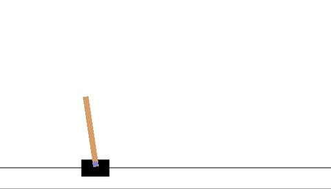
CartPole-v0 environment: OpenAI Gym
Google DeepMind has devised a solid algorithm for tackling the continuous action space problem. Building off the prior work of [2] on Deterministic Policy Gradients, they have produced a policy-gradient actor-critic algorithm called Deep Deterministic Policy Gradients (DDPG) [4] that is off-policy and model-free, and that uses some of the deep learning tricks that were introduced along with Deep Q-Networks (hence the “deep”-ness of DDPG). In this blog post, we’re going to discuss how to implement this algorithm using Tensorflow and tflearn, and then evaluate it with OpenAI Gym on the pendulum environment. I’ll also discuss some of the theory behind it. Regrettably, I can’t start with introducing the basics of reinforcement learning since that would make this blog post much too long; however, Richard Sutton’s book (linked above), as well as David Silver’s course, are excellent resources to get going with RL.
Lets Start With Some Theory
[Wait, I just want to skip to the Tensorflow part!]
Policy-Gradient Methods
Policy-Gradient (PG) algorithms optimize a policy end-to-end by computing noisy estimates of the gradient of the expected reward of the policy and then updating the policy in the gradient direction. Traditionally, PG methods have assumed a stochastic policy $\mu (a | s)$, which gives a probability distribution over actions. Ideally, the algorithm sees lots of training examples of high rewards from good actions and negative rewards from bad actions. Then, it can increase the probability of the good actions. In practice, you tend to run into plenty of problems with vanilla-PG; for example, getting one reward signal at the end of a long episode of interaction with the environment makes it difficult to ascertain exactly which action was the good one. This is known as the credit assignment problem. For RL problems with continuous action spaces, vanilla-PG is all but useless. You can, however, get vanilla-PG to work with some RL domains that take in visual inputs and have discrete action spaces with a convolutional neural network representing your policy (talk about standing on the shoulders of giants!). There are extensions to the vanilla-PG algorithm such as REINFORCE and Natural Policy Gradients that make the algorithm much more viable. For a first look into stochastic policy gradients, you can find an overview of the Stochastic Policy Gradient theorem in [2], an in-depth blog post by Andrej Karpathy on here.
Actor-Critic Algorithms

The actor-critic architecture, figure from [1]
The Actor-Critic learning algorithm is used to represent the policy function independently of the value function. The policy function structure is known as the actor, and the value function structure is referred to as the critic. The actor produces an action given the current state of the environment, and the critic produces a TD (Temporal-Difference) error signal given the state and resultant reward. If the critic is estimating the action-value function $Q(s,a)$, it will also need the output of the actor. The output of the critic drives learning in both the actor and the critic. In Deep Reinforcement Learning, neural networks can be used to represent the actor and critic structures.
Off-Policy vs. On-Policy
Reinforcement Learning algorithms which are characterized as off-policy generally employ a separate behavior policy that is independent of the policy being improved upon; the behavior policy is used to simulate trajectories. A key benefit of this separation is that the behavior policy can operate by sampling all actions, whereas the estimation policy can be deterministic (e.g., greedy) [1]. Q-learning is an off-policy algorithm, since it updates the Q values without making any assumptions about the actual policy being followed. Rather, the Q-learning algorithm simply states that the Q-value corresponding to state $s(t)$ and action $a(t)$ is updated using the Q-value of the next state $s(t + 1)$ and the action $a(t + 1)$ that maximizes the Q-value at state $s(t + 1)$.
On-policy algorithms directly use the policy that is being estimated to sample trajectories during training.
Model-free Algorithms
Model-free RL algorithms are those that make no effort to learn the underlying dynamics that govern how an agent interacts with the environment. In the case where the environment has a discrete state space and the agent has a discrete number of actions to choose from, a model of the dynamics of the environment is the 1-step transition matrix: $T(s(t + 1)|s(t), a(t))$. This stochastic matrix gives all of the probabilities for arriving at a desired state given the current state and action. Clearly, for problems with high-dimensional state and action spaces, this matrix is incredibly expensive in space and time to compute. If your state space is the set of all possible 64 x 64 RGB images and your agent has 18 actions available to it, the transition matrix’s size is $|S \times S \times A| \approx |(68.7 \times 10^{9}) \times (68.7 \times 10^9) \times 18|$, and at 32 bits per matrix element, thats around $3.4 \times 10^{14}$ GB to store it in RAM!
Rather than dealing with all of that, model-free algorithms directly estimate the optimal policy or value function through algorithms such as policy iteration or value iteration. This is much more computationally efficient. I should note that, if possible, obtaining and using a good approximation of the underlying model of the environment can only be beneficial. Be wary- using a bad approximation of a model of the environment will only bring you misery. Just as well, model-free methods generally require a larger number of training examples.
The Meat and Potatoes of DDPG
At its core, DDPG is a policy gradient algorithm that uses a stochastic behavior policy for good exploration but estimates a deterministic target policy, which is much easier to learn. Policy gradient algorithms utilize a form of policy iteration: they evaluate the policy, and then follow the policy gradient to maximize performance. Since DDPG is off-policy and uses a deterministic target policy, this allows for the use of the Deterministic Policy Gradient theorem (which will be derived shortly). DDPG is an actor-critic algorithm as well; it primarily uses two neural networks, one for the actor and one for the critic. These networks compute action predictions for the current state and generate a temporal-difference (TD) error signal each time step. The input of the actor network is the current state, and the output is a single real value representing an action chosen from a continuous action space (whoa!). The critic’s output is simply the estimated Q-value of the current state and of the action given by the actor. The deterministic policy gradient theorem provides the update rule for the weights of the actor network. The critic network is updated from the gradients obtained from the TD error signal.
Sadly, it turns out that tossing neural networks at DPG results in an algorithm that behaves poorly, resisting all of your most valiant efforts to get it to converge. The following are most likely some of the key conspirators:
-
In general, training and evaluating your policy and/or value function with thousands of temporally-correlated simulated trajectories leads to the introduction of enormous amounts of variance in your approximation of the true Q-function (the critic). The TD error signal is excellent at compounding the variance introduced by your bad predictions over time. It is highly suggested to use a replay buffer to store the experiences of the agent during training, and then randomly sample experiences to use for learning in order to break up the temporal correlations within different training episodes. This technique is known as experience replay. DDPG uses this.
-
Directly updating your actor and critic neural network weights with the gradients obtained from the TD error signal that was computed from both your replay buffer and the output of the actor and critic networks causes your learning algorithm to diverge (or to not learn at all). It was recently discovered that using a set of target networks to generate the targets for your TD error computation regularizes your learning algorithm and increases stability. Accordingly, here are the equations for the TD target $y_i$ and the loss function for the critic network:
Here, a minibatch of size $N$ has been sampled from the replay buffer, with the $i$ index referring to the i’th sample. The target for the TD error computation, $y_i$, is computed from the sum of the immediate reward and the outputs of the target actor and critic networks, having weights $\theta^{\mu’}$ and $\theta^{Q’}$ respectively. Then, the critic loss can be computed w.r.t. the output $Q(s_i, a_i | \theta^{Q})$ of the critic network for the i’th sample.
See [3] for more details on the use of target networks.
Now, as mentioned above, the weights of the critic network can be updated with the gradients obtained from the loss function in Eq. 2. Also, remember that the actor network is updated with the Deterministic Policy Gradient. Here lies the crux of DDPG! Silver, et al., [2] proved that the stochastic policy gradient $\nabla_{\theta} \mu (a | s, \theta)$, which is the gradient of the policy’s performance, is equivalent to the deterministic policy gradient, which is given by:
\[\begin{equation} \nabla_{\theta^{\mu}} \mu \approx \mathbb{E}_{\mu'} \big [ \nabla_{a} Q(s, a|\theta^{Q})|_{s=s_t,a=\mu(s_t)} \nabla_{\theta^{\mu}} \mu(s|\theta^{\mu})|_{s=s_t} \big ] \end{equation}\]Notice that the policy term in the expectation is not a distribution over actions. It turns out that all you need is the gradient of the output of the critic network w.r.t. the actions, multiplied by the gradient of the output of the actor network w.r.t. its parameters, averaged over a minibatch. Simple!
I think the proof of the deterministic policy gradient theorem is quite illuminating, so I’d like to demonstrate it here before moving on to the code.
The expectation in the right-hand side of Eq. 6 is exactly what we want. In [3], it is shown that the stochastic policy gradient converges to Eq. 4 in the limit as the variance of the stochastic policy gradient approaches 0. This is significant because it allows for all of the machinery for stochastic policy gradients to be applied to deterministic policy gradients.
Enough With The Chit Chat, Let’s See Some Code!
Let’s get started.
We’re writing code to solve the Pendulum environment in OpenAI gym, which has a low-dimensional state space and a single continuous action within [-2, 2]. The goal is to swing up and balance the pendulum.

The first part is easy. Set up a data structure to represent your replay buffer. I recommend using a deque from python’s collections library. The replay buffer will return a randomly chosen batch of experiences when queried.
from collections import deque
import random
import numpy as np

class ReplayBuffer(object):

    def __init__(self, buffer_size):
        self.buffer_size = buffer_size
        self.count = 0
        self.buffer = deque()

    def add(self, s, a, r, t, s2):
        experience = (s, a, r, t, s2)
        if self.count < self.buffer_size:
            self.buffer.append(experience)
            self.count += 1
        else:
            self.buffer.popleft()
            self.buffer.append(experience)

    def size(self):
        return self.count

    def sample_batch(self, batch_size):
        '''
        batch_size specifies the number of experiences to add
        to the batch. If the replay buffer has less than batch_size
        elements, simply return all of the elements within the buffer.
        Generally, you'll want to wait until the buffer has at least
        batch_size elements before beginning to sample from it.
        '''
        batch = []

        if self.count < batch_size:
            batch = random.sample(self.buffer, self.count)
        else:
            batch = random.sample(self.buffer, batch_size)

        s_batch = np.array([_[0] for _ in batch])
        a_batch = np.array([_[1] for _ in batch])
        r_batch = np.array([_[2] for _ in batch])
        t_batch = np.array([_[3] for _ in batch])
        s2_batch = np.array([_[4] for _ in batch])

        return s_batch, a_batch, r_batch, t_batch, s2_batch

    def clear(self):
        self.buffer.clear()
        self.count = 0
Okay, lets define our actor and critic networks. We’re going to use tflearn to condense the boilerplate code.
class ActorNetwork(object):

    ...

    def create_actor_network(self):
        inputs = tflearn.input_data(shape=[None, self.s_dim])
        net = tflearn.fully_connected(inputs, 400)
        net = tflearn.layers.normalization.batch_normalization(net)
        net = tflearn.activations.relu(net)
        net = tflearn.fully_connected(net, 300)
        net = tflearn.layers.normalization.batch_normalization(net)
        net = tflearn.activations.relu(net)
        # Final layer weights are init to Uniform[-3e-3, 3e-3]
        w_init = tflearn.initializations.uniform(minval=-0.003, maxval=0.003)
        out = tflearn.fully_connected(
            net, self.a_dim, activation='tanh', weights_init=w_init)
        # Scale output to -action_bound to action_bound
        scaled_out = tf.multiply(out, self.action_bound)
        return inputs, out, scaled_out


class CriticNetwork(object):

    ...

    def create_critic_network(self):
        inputs = tflearn.input_data(shape=[None, self.s_dim])
        action = tflearn.input_data(shape=[None, self.a_dim])
        net = tflearn.fully_connected(inputs, 400)
        net = tflearn.layers.normalization.batch_normalization(net)
        net = tflearn.activations.relu(net)

        # Add the action tensor in the 2nd hidden layer
        # Use two temp layers to get the corresponding weights and biases
        t1 = tflearn.fully_connected(net, 300)
        t2 = tflearn.fully_connected(action, 300)

        net = tflearn.activation(
            tf.matmul(net, t1.W) + tf.matmul(action, t2.W) + t2.b, activation='relu')

        # linear layer connected to 1 output representing Q(s,a)
        # Weights are init to Uniform[-3e-3, 3e-3]
        w_init = tflearn.initializations.uniform(minval=-0.003, maxval=0.003)
        out = tflearn.fully_connected(net, 1, weights_init=w_init)
        return inputs, action, out
I would suggest placing these two functions in separate Actor and Critic classes, as shown above. The hyperparameter and layer details for the networks are in the appendix of the DDPG paper [4]. The networks for the low-dimensional state-space problems are pretty simple, though. For the actor network, the output is a tanh layer scaled to be between $[-b, +b], b \in \mathbb{R}$. This is useful when your action space is on the real line but is bounded and closed, as is the case for the pendulum task.
Notice that the critic network takes both the state and the action as inputs; however, the action input skips the first layer. This is a design decision that has experimentally worked well. Accommodating this with tflearn was a bit tricky.
Make sure to use Tensorflow placeholders, created by tflearn.input_data, for the inputs. Leaving the first dimension of the placeholders as None allows you to train on batches of experiences.
You can simply call these creation methods twice, once to create the actor and critic networks that will be used for training, and again to create your target actor and critic networks.
You can create a Tensorflow Op to update the target network parameters like so:
self.network_params = tf.trainable_variables()

self.target_network_params = tf.trainable_variables()[len(self.network_params):]

# Op for periodically updating target network with online network weights
self.update_target_network_params = \
    [self.target_network_params[i].assign(tf.mul(self.network_params[i], self.tau) + \
        tf.mul(self.target_network_params[i], 1. - self.tau))
        for i in range(len(self.target_network_params))]
This looks a bit convoluted, but it’s actually a great display of Tensorflow’s flexibility. You’re defining a Tensorflow Op, update_target_network_params, that will copy the parameters of the online network with a mixing factor $\tau$. Make sure you’re copying over the correct Tensorflow variables by checking what is being returned by tf.trainable_variables(). You’ll need to define this Op for both the actor and critic.
Let’s define the gradient computation and optimization Tensorflow operations. We’ll use ADAM as our optimization method. It’s sort of replaced SGD as the de-facto standard, now that it’s implemented in so many plug-and-play deep-learning libraries such as tflearn and keras and tends to outperform it.
For the actor network…
# This gradient will be provided by the critic network
self.action_gradient = tf.placeholder(tf.float32, [None, self.a_dim])

# Combine the gradients, dividing by the batch size to
# account for the fact that the gradients are summed over the
# batch by tf.gradients
self.unnormalized_actor_gradients = tf.gradients(
    self.scaled_out, self.network_params, -self.action_gradient)
self.actor_gradients = list(map(lambda x: tf.div(x, self.batch_size), self.unnormalized_actor_gradients))

# Optimization Op
self.optimize = tf.train.AdamOptimizer(self.learning_rate).\
    apply_gradients(zip(self.actor_gradients, self.network_params))
Notice how the gradients are combined. tf.gradients() makes it quite easy to implement the Deterministic Policy Gradient equation (Eq. 4). I negate the action-value gradient since we want the actor to follow the action-value gradients. Tensorflow will take the sum and average of the gradients of your minibatch.
Then, for the critic network…
# Network target (y_i)
# Obtained from the target networks
self.predicted_q_value = tf.placeholder(tf.float32, [None, 1])

# Define loss and optimization Op
self.loss = tflearn.mean_square(self.predicted_q_value, self.out)
self.optimize = tf.train.AdamOptimizer(self.learning_rate).minimize(self.loss)

# Get the gradient of the net w.r.t. the action
self.action_grads = tf.gradients(self.out, self.action)
This is exactly Eq. 2. Make sure to grab the action-value gradients at the end there to pass to the policy network for gradient computation.
I like to encapsulate calls to my Tensorflow session to keep things organized and readable in my training code. For brevity’s sake, I’ll just show the ones for the actor network.
...

def train(self, inputs, a_gradient):
    self.sess.run(self.optimize, feed_dict={
        self.inputs: inputs,
        self.action_gradient: a_gradient
    })

def predict(self, inputs):
    return self.sess.run(self.scaled_out, feed_dict={
        self.inputs: inputs
    })

def predict_target(self, inputs):
    return self.sess.run(self.target_scaled_out, feed_dict={
        self.target_inputs: inputs
    })

def update_target_network(self):
    self.sess.run(self.update_target_network_params)

...
Now, lets show the main training loop and we’ll be done!
# Constants
TAU = 0.001
ACTOR_LEARNING_RATE = 0.0001
CRITIC_LEARNING_RATE = 0.001
BUFFER_SIZE = 1000000
MINIBATCH_SIZE = 64
MAX_EPISODES = 50000
MAX_EP_STEPS = 1000
GAMMA = 0.99
...

with tf.Session() as sess:

    env = gym.make('Pendulum-v0')

    state_dim = env.observation_space.shape[0]
    action_dim = env.action_space.shape[0]
    action_bound = env.action_space.high
    # Ensure action bound is symmetric
    assert (env.action_space.high == -env.action_space.low)

    actor = ActorNetwork(sess, state_dim, action_dim, action_bound, \
        ACTOR_LEARNING_RATE, TAU)

    critic = CriticNetwork(sess, state_dim, action_dim, \
        CRITIC_LEARNING_RATE, TAU, actor.get_num_trainable_vars())

    actor_noise = OrnsteinUhlenbeckActionNoise(mu=np.zeros(action_dim))

    # Initialize our Tensorflow variables
    sess.run(tf.initialize_all_variables())

    # Initialize target network weights
    actor.update_target_network()
    critic.update_target_network()

    # Initialize replay memory
    replay_buffer = ReplayBuffer(BUFFER_SIZE)

    for i in range(MAX_EPISODES):

        s = env.reset()

        for j in range(MAX_EP_STEPS):

            if RENDER_ENV:
                env.render()

            # Added exploration noise. In the literature, they use
            # the Ornstein-Uhlenbeck stochastic process for control tasks
            # that deal with momentum
            a = actor.predict(np.reshape(s, (1, actor.s_dim))) + actor_noise()

            s2, r, terminal, info = env.step(a[0])

            replay_buffer.add(np.reshape(s, (actor.s_dim,)), np.reshape(a, (actor.a_dim,)), r, \
                terminal, np.reshape(s2, (actor.s_dim,)))

            # Keep adding experience to the memory until
            # there are at least minibatch size samples
            if replay_buffer.size() > MINIBATCH_SIZE:
                s_batch, a_batch, r_batch, t_batch, s2_batch = \
                    replay_buffer.sample_batch(MINIBATCH_SIZE)

                # Calculate targets
                target_q = critic.predict_target(s2_batch, actor.predict_target(s2_batch))

                y_i = []
                for k in range(MINIBATCH_SIZE):
                    if t_batch[k]:
                        y_i.append(r_batch[k])
                    else:
                        y_i.append(r_batch[k] + GAMMA * target_q[k])

                # Update the critic given the targets
                predicted_q_value, _ = critic.train(s_batch, a_batch, np.reshape(y_i, (MINIBATCH_SIZE, 1)))

                # Update the actor policy using the sampled gradient
                a_outs = actor.predict(s_batch)
                grads = critic.action_gradients(s_batch, a_outs)
                actor.train(s_batch, grads[0])

                # Update target networks
                actor.update_target_network()
                critic.update_target_network()

            if terminal:
                break
You’ll want to add book-keeping to the code and arrange things a little more neatly- you can find the full code here.
I used Tensorboard to view the total reward per episode and average max Q. Tensorflow is a bit low-level, so it’s definitely recommended to use wrappers like tflearn, keras, Tensorboard, etc., on top of it. I am quite pleased with TF though; it’s no surprise that it got so popular so quickly.
Looking Forward
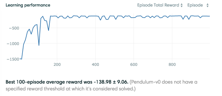
Results from running the code on Pendulum-v0
Despite the fact that I ran this code on the courageous CPU of my Macbook Air, it converged relatively quickly to a good solution. Some ways to potentially get better performance (besides running the code on a GPU lol):
-
Use a priority algorithm for sampling from the replay buffer instead of uniformly sampling. See my summary of Prioritized Experience Replay.
-
Experiment with different stochastic policies to improve exploration.
-
Use recurrent networks to capture temporal nuances within the environment.
The authors of DDPG also used convolutional neural networks to tackle control tasks of higher complexities. They were able to learn good policies with just pixel inputs, which is really cool.
References
- Sutton, Richard S., and Andrew G. Barto. Reinforcement learning: An introduction.
- Silver, et al. Deterministic Policy Gradients
- Mnih, et al. Human-level control through deep reinforcement learning
- Lillicrap, et al. Continuous control with Deep Reinforcement Learning