MLSS 2019

Now that the 2019 London MLSS is over, I thought I’d share a couple things about my experience and summarize some of the fascinating technical content I learned over the 10 days of lectures. This will not only help improve my recall of the material, but will also make it easy to share some of what I learned with my lab and with others that weren’t able to attend. If you find any mistakes, please feel free to reach out so I can make corrections. :)

First and foremost, however, let me send a huge thank you to the organizers, Arthur Gretton and Marc Deisenroth, for putting this amazing event together. It was an incredibly rewarding experience for me. Also, thank you to all the lecturers and volunteers as well!

Before I jump into discussing technical highlights…

Wait, why are PhD students going to summer school?

For those of you reading this that may not know what a summer school is, summer schools are typically focused on a specific topic, have daily lectures and practicals, and can last from a few days to two weeks. The location of the summer school is usually in an exciting place, so that students can explore the area together. Usually there’s also a poster session for students to share their ongoing work. At this MLSS, days were structured as two 2-hour lectures followed by a practical which involved writing code for some exercises.

From what I’ve been told and from what I experienced, one of the best reason to attend a summer school is to make friends with other highly-motivated students from around the world. We were lucky enough that Arthur and Marc assembled an amazingly diverse cohort. Out of the ~200 students that attended, 53 nationalities were represented!

It wasn’t all work

I was surrounded by a ton of brilliant people from the moment I arrived in London. Here are some highlights from the fun times we had:

Experienced the hottest day in UK history. OK so this wasn’t “fun” but our joint suffering was a great bonding experience. I’m used to this type of heat back in Florida, but in London most buildings don’t have air conditioning.
On the Saturday afternoon we bought ~half the food at a local grocery store to feed a large group of us that were having a picnic in Green park near Buckingham Palace
A group of us saw A Midsummer’s Night Dream at the Open Air Theatre in Regent’s Park

After our tour of the Tower of London

Technical highlights from MLSS

I’ll only be discussing some of the lectures in this post, but all of the slides and lectures are available at the MLSS Github page.

Optimization

Lecturer: John Duchi [Slides] [Video 1] [Video 2]

John first introduced to us the main ideas in convex optimization and then covered some special topics. A big takeaway from his lecture is to stop and think about each particular optimization problem for a bit instead of just tossing SGD at it (supposedly we shouldn’t say “SGD” because the trajectory taken by stochastic gradient methods like “SGD” don’t strictly “descend”, rather they wander around quite a bit). His point is that we can do a lot better.

The concepts of subgradients and a subdifferential were new to me. A vector $g$ is a subgradient of a function $f$ at $x$ if $f(y) \geq f(x) + <g, y - x>.$

In a picture:

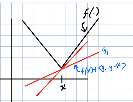
A subgradient of the absolute value function

The subdifferential is the set of all vectors $g$ that satisfy the above inequality. These are useful because they can be computed so long as $f$ can be evaluated, which means we can derive optimization algorithms in terms of subgradients to make them more broadly applicable.

Another new concept was the notion of $\rho$-weakly convex functions. We learned that regularizing your function to make it sort-of convex by adding a large quadratic to it results in what is known as a $\rho$-weakly convex function.

Ultimately, John gave us three steps to follow:

Make a local approximation to your function
Add regularization to “avoid bouncing around like an idiot”
Optimize approximately

Additional Resources

Interpretability

Lecturer: Sanmi Koyejo [Slides] [Video 1] [Video 2]

Key takeaways:

When building an ML system for a task where the repercussions of false positives/false negatives are unknown, it is usually best to defer decision-making to someone downstream
Monotonicity as an interpretability criterion: if feature $X$ “increases”, the output should “increase” as well
A standard definition of what it means for a model to be “interpretable” is still missing

Additional Resources

Gaussian Processes

Lecturer: James Hensman [Slides] [Video 1] [Video 2]

GPs have always been a bit mind-boggling to me. Good thing MLSS was held in the UK, where there seems to be a high concentration of GP/Bayesian ML researchers. Also, James’ slides contain amazing visuals.

What’s a GP? As Mackay puts it, GPs are smoothing techniques that involve placing a Gaussian prior over the functions in the hypothesis class.

I highly recommend checking out Lab 0 and Lab 1 from the GP practical here which were great for building the intuitions.

Multivariate normals

GPs heavily make use of multivariate normal distributions (MVN). In fact, GPs are based on infinite-dimensional MVNs… It took a while for me to wrap my head around this, but these plots from James’ slides really helped:

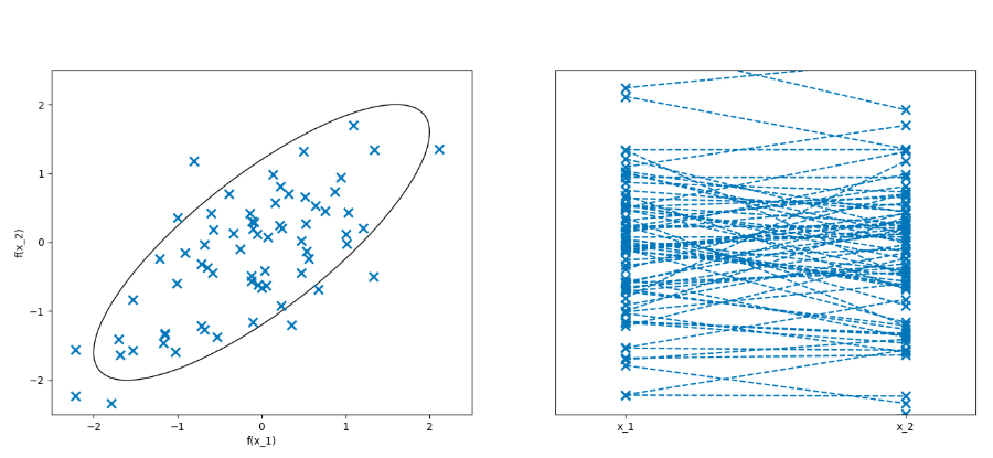
samples from a 2D MVN. See slides for GIF versions.

The plot on the RHS is the important one. The x-axis represents the two dimensions of this MVN; there are no units for the x-axis, it simply depicts each of the N dimensions of an MVN from 1 to N (the order matters!). The y-axis depicts the values of a random variate sampled from this MVN. A line is drawn connecting $f(x_1)$ to $f(x_2)$. For a 6D MVN, there would be 6 ticks on the x-axis and a line connecting all 6 function values. The trick with GPs is that we (theoretically) let the number of dimensions go to infinity, so the x-axis becomes a continuum. But in practice, we only have a finite number of data points, and we assume the $(x_i, f(x_i))$ pairs are observations of this unknown function.

Confused? Let’s take a step back. In Lab 0, we build some intuition by looking at Linear Regression and then the extension to Bayesian Linear Regression. For GP regression, we make the usual assumption that some unknown target function generated our data, except now our hypothesis class is much more expressive. GPs place a prior over the functions in the hypothesis class. They do this by defining a (Gaussian) stochastic process indexed by the data points:

\[p\Biggl(\begin{bmatrix} f(x_1)\\ f(x_2) \\ \cdots \\ f(x_n) \end{bmatrix} \Biggr) = \mathscr{N} \Biggl( \begin{bmatrix} \mu(x_1)\\ \mu(x_2) \\ \cdots \\ \mu(x_n) \end{bmatrix}, \begin{bmatrix} k(x_1, x_1) & \cdots & k(x_1,x_n)\\ \vdots & & \vdots \\ k(x_n, x_1) & \cdots & k(x_n, x_n)\end{bmatrix} \Biggr).\]

Covariance functions

Note that we can usually transform our data to be zero-mean, so the mean function $\mathbf{\mu}$ is generally assumed to be $0$ and our main concern is the kernel matrix $K$, also known as the gram matrix. $K$ is the covariance function of the GP. Unlike regular (Bayesian) Linear Regression, GPs have a certain useful structure that comes with formulating the problem as a (Gaussian) stochastic process. That is, the kernel matrix $K$ enables us to incorporate prior knowledge about how we expect the data points to interact. In the next section, I’ll take about kernels and the kernel matrix $K$ in more detail.

Once we have the basic machinery of GPs down, we can do some cool stuff like compute the conditional distribution of the function that fits a test point $x^*$ given a training set of point pairs $(x_i, f(x_i))$.

We also covered model selection using the marginal likelihood of a GP. Kernels are typically parameterized by a lengthscale and variance parameter, and the marginal likelihood objective for selecting these kernel parameters nicely trades off model complexity with data fit.

Finally, I’ll briefly mention something we touched on at the end of the GP lecture that was interesting. Since GPs require inverting $K$ to do inference, sparse GPs cleverly select a small set of “pseudo-inputs” that approximate the original GP well and allow for using GPs on much larger datasets.

GPs are useful in modern ML because many problems are concerned with interpolating a function given noisy observations using a Bayesian approach.

Additional Resources

Kernels

Lecturer: Lorenzo Rosasco [Slides] [Video 1] [Video 2]

You may have heard of the kernel trick, which involves replacing all inner products of features in an algorithm with a kernel evaluation, e.g., as in Kernel K-Means.

More than just a trick

Lorenzo showed us some recent work he’s been doing on scaling up kernel methods to the sizes of datasets commonly consumed by deep learning. To do this type of research, it is important to understand the theory of kernel methods. We covered some of this during the lecture, like Reproducing Kernel Hilbert Spaces (RKHSs). I think this lecture was one of the most difficult to swallow in the time allotted from the entire MLSS.

RKHS

Here is my attempt to summarize my understanding of RKHSs. Please see Arthur’s notes (linked below), especially Section 4.1, for a great explanation.

An RKHS is an abstract mathematical space closely intertwined with the notion of kernels. An RKHS is an extension of a Hilbert space; that is, it has all of the properties of a Hilbert space (it’s a vector space, has an inner product, and is complete), plus two other key properties. Note that RKHSs are function spaces; the primitive object that lives in an RKHS is a function.

In fact, evaluating a function in the RKHS maps points from $\mathscr{X} \rightarrow \mathbb{R}$, where $\mathscr{X}$ is the data. However, the “representation” of a function in the RKHS could be an infinite-dimensional vector, if the feature maps corresponding to a particular kernel are infinite dimensional. Since we care about the inner product (evaluation) of the functions in the RKHS, we never actually have to deal with these individual, potentially infinite-dimensional representations. This took me a long time to wrap my head around (see Lemma 9 in Arthur’s notes).

To my understanding, the fact that certain kernels (e.g., the RBF kernel) are said to lift your original feature space to an “infinite-dimensional feature space” comes from the fact that such a kernel is defined as an infinite series of inner products of the original features. This is valid when the series converges (the assumption here is that each feature map is in L2).

If we are given an RKHS, then the key tool we can leverage, which comes for free with the RKHS, is the reproducing property of said RKHS. The reproducing property of the RKHS says that the evaluation of any function in the RKHS at a point $x \in \mathscr{X}$ is the inner product of the function with the corresponding reproducing kernel of the RKHS at the point. The Riesz representation theorem guarantees for us that such a reproducing kernel exists.

Lorenzo showed us how we can start with feature maps and arrive at RKHSs. That is, if you aren’t given an RKHS, you can instead start by defining a kernel as the inner product $k(x,y) := \langle \phi(x), \phi(y) \rangle$ between feature maps. Equivalently, we can define a kernel as a symmetric, positive definite function $k : \mathscr{X} \times \mathscr{X} \rightarrow \mathbb{R}$, and a theorem (Moore-Aronszajn) tells us that there’s a corresponding RKHS for which $k$ is a reproducing kernel. However, in the latter case, there are infinitely many feature maps corresponding to the symmetric, positive definite function we started with.

Additional Resources

MCMC

Lecturer: Michael Betancourt [Slides] [Video 1] [Video 2]

What is Bayesian computation?

Specify a model
Compute posterior expectation values

The first part of our MCMC lecture was all about having us update our mental priors about high-dimensional statistics. For example, although we may think that the mode of a probability density contributes most to an integral when integrating over parameter space, this falls apart quickly in higher dimensions. This is because the relative amount of volume the mode occupies in high dimensions rapidly disappears ($d\theta \approx 0$), so that wherever the majority of the probability mass is sitting and occupying a non-trivial amount of volume ($d\theta$ » $0$) contributes most to the integral. We learned that probability mass concentrates on a thin and hard to find hypersurface called the typical set in higher dimensions.

What about variational methods?

Variational inference, which replaces integration with an optimization problem and makes simplistic assumptions about the variational posterior, underestimates the variance and favors solutions that land inside the target typical set. Yikes!

Markov chains

Monte carlo methods use samples from the exact target typical set. Markov chains are great because a Markov transition that targets a particular distribution will naturally concentrate towards its probability mass. In practice for MCMC, Michael showed us that the chain quickly converges onto the typical set. The main challenge of MCMC methods seem to be handling various failure modes that cause divergence or cases where the chain gets stuck somewhere within the typical set.

Diagnosing your MCMC

From the law of large numbers, we get that Markov chains are asymptotically consistent estimators. However, due to various pathologies, we need more sophisticated diagnostic tools and algorithms to get good finite time behavior. One diagnostic tool is the effective sample size (ESS). The more anti-correlated the samples from the Markov chain are, the higher the ESS.

A robust strategy is to run multiple chains from various initial states and compare the expectations. Another strategy is to check the potential scale reduction factor, or R-hat, which is similar to an ANOVA between multiple chains.

Hamiltonian Monte Carlo

HMC is an alternative to Metropolis-Hastings MCMC. One issue with MH is that a naive Normal proposal density will almost always jump outside of the typical set, because most of the volume lies outside. Lowering the std dev of the proposal to avoid this means convergence will be too slow.

We want to efficiently explore the typical set without leaving it. Insight: align a vector field to the typical set and then integrate along the field. HMC is the formal procedure for adding just enough momentum to the gradient vector field to align the gradient field with the typical set. The analogy Michael used is that we need to add the momentum needed for a satellite to enter orbit around the earth.

How to do this? Use Hamiltonian measure-preserving flow, which is a scalar function $H(p,q)$ of the parameters $q$ and momentum $p$ such that $H(p,q) = -log (\pi(p|q)) -\log (\pi(q))$. Here, $\pi(q)$ is the target density, which is specified by the problem. $\pi(p|q)$ is a conditional density for the momentum, which we choose. According to Michael, this is the only way of producing the gradient vector field we want to integrate along that actually works (this is a magic, hand-wavy thing).

The Markov transitions now consist of randomly sampling a Hamiltonian trajectory. Motion is governed by the above Hamiltonian, which has a kinetic and potential energy term. From the current location on the typical set, we randomly sample the momentum and the trajectory length, and then use an ODE numerical integrator to compute where we end up. I picture this like a marble being released with some initial momentum inside a bowl-shaped surface; wherever the marble finally rests after rolling around for a while is analogous to the next sample from the posterior we draw and is the next state of the chain.

Numerical integration introduces some errors, so we have to be careful about the type of integration we use and how we correct for the introduced bias in our estimator. Use Stan in practice for your MCMC needs.

Additional Resources

Fairness

Lecturer: Timnit Gebru [Slides] [Video]

Timnit gave an incredibly engaging lecture, which also doubled as a nice break from brain-bending equations. Here are some key takeaways:

Timnit talked about “Fairwashing”, which is also discussed by Zachary Lipton in his recent TWiML interview. Basically, it is not enough to take a contentious research topic and simply try to “make it fair”. The idea of “make X fair” misses the point: we need to step back and critically consider the implications of doing the research in the first place. Ask: should we even be building this technology? And then the follow-up questions: if we don’t, will someone else build it anyways? If so, what do we do?

We learned about her PhD project where they took Google street view images and ran computer vision data mining on images of cars to extract patterns about the US population. Since I grew up in Jacksonville, FL, I thought I’d include this slide showing that it is the 10th most segregated city (measured by disparity in average car prices) in the US. Yikes!

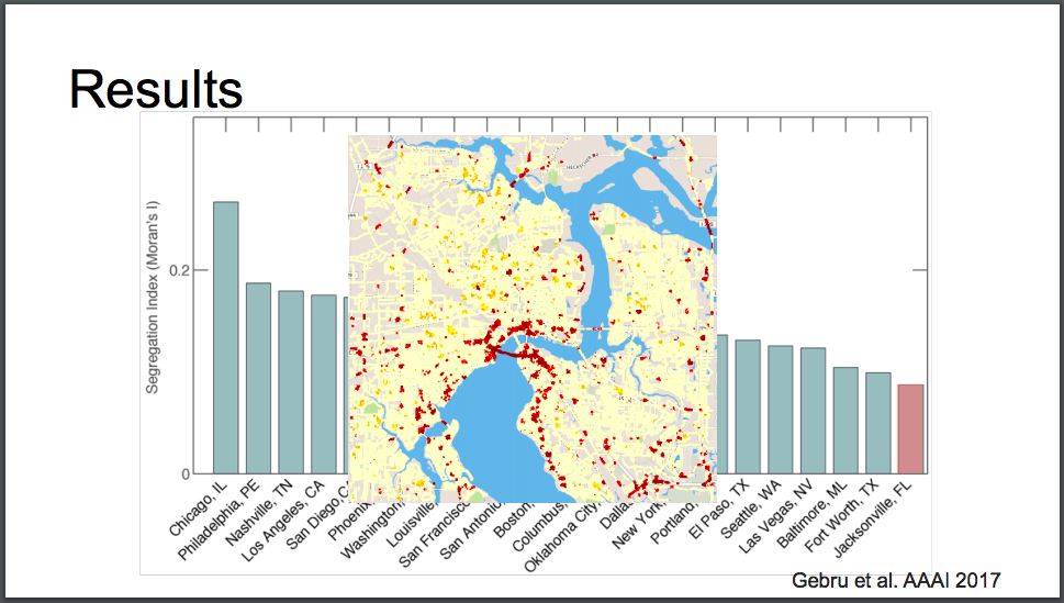
The red in the center is San Marco/Riverside. Duuuval

When the data is biased (and data collected out in the real world reflects the current state of the society from which it was extracted from), model predictions will be biased. Some examples we saw: using ML to predict who to hire, placing current ML techniques in the hands of ICE, predictive policing, gender classification, and facial recognition.

Science is inherently political. We all have a responsibility to be cognizant of the dual-use nature of the technologies we create. Even people working on “theory” must adhere to this. The people working on the foundations of our modern statistics (like Fisher) were eugenicists!

Additional Resources

Submodularity

Lecturer: Stefanie Jegelka [Slides] [Video]

This was a fairly niche topic and most people hadn’t heard of it. Essentially, it is a technique in combinatorial optimization for optimal subset selection. Subset selection is clearly relevant to ML, e.g., for active learning, coordinate selection, compression, and so on. However, optimizing a set function over subsets $F(s), s \subseteq S$ is non-trivial; sets are discrete objects, and for any set $S$ there are $2^S$ possible subsets!

It turns out there are specific classes of functions called submodular functions that can be optimized in a reasonable amount of time. These functions have a property called submodularity. In words, this means that if you have a subset $T$ and a subset $S$, and $T \subseteq S$, adding a new element $a \notin S$ to the “smaller” subset $T$ should give you a higher value than adding it to $S$. This is also referred to as diminishing gains. Written out, it is

\[F(T \cup \{a\}) - F(T) \geq F(S \cup \{a\}) - F(S), T \subseteq S, a \notin T.\]

You can also think about $F$ like a concave function, such that its “discrete derivative” is non-increasing.

An example of a submodular function is the coverage function: given $A_1, …, A_n \subset U$,

\[F(S) = \Bigl | \bigcup_{j \in S} A_j \Bigr |.\]

As your coverage $|S|$ increases, the increase in the number of subsets in the union achieved by adding another index $j’$ to $S$ will be smaller.

Convex or concave?

It is not obvious whether submodular functions are more like convex or concave functions, as they share similarities with both. The fact that there are similarities hints at the reason why they are interesting, since convex and concave functions are “nice” to optimize in continuous optimization. We already mentioned the non-increasing discrete derivative property, which is similar to concave functions. The similarity to convexity comes from the fact that it is easier to minimize a submodular function than it is to maximize one (e.g., Max Cut; this is NP-Hard).

Greedy algorithms

We discussed greedy algorithms for maximizing submodular functions during the lecture. The basic algorithm for finding

$\max_{S} F(S) \texttt{ s.t. } |S| \leq k$ is as follows:

$S_0 = \emptyset$
$\texttt{for } i=1,…,k-1$
1. $e^* = \texttt{arg max}_{e \in \mathscr{V} \setminus S_i} F(S_i \cup {e})$
2. $S_{i+1} = S_i \cup {e^*}$

This works because $F$ is submodular - the marginal improvement of adding a single item gives information about the global value. Furthemore, $F$ is monotonic in that adding items can never reduce $F$. Lots more on this in the slides.

Continuous relaxation for minimization

What if we want to minimize a submodular function? We can consider a continuous relaxations of $F$ to a convex function. The Lovasz extension provides a method for relaxing a function defined on the Boolean hypercube to $[0,1]^N$. The result is a piece-wise, linear convex function $f(z)$ that can be optimized using subgradient methods, and a final result can be obtained by rounding.