Linear Least-Squares Algorithms for Temporal Difference Learning
Summary
A Brief Description of TD($\lambda$)
In TD($\lambda$), a parameterized linear function approximator is used to represent the value function. The parameter update for vector $\theta_{t}$ is:
\[\begin{equation} \theta_{t+1} = \theta_{t} + \alpha_{\eta(x_{t})} \big [ R_{t} + \gamma V_{t}(x_{t+1} - V_{t} \big ] \sum_{k=1}^{t} \lambda^{t-k} \nabla_{\theta_{t}} V_{t}(x_k) \end{equation}\]$\alpha_{\eta(x_{t})}$ is the step-size parameter, and $\eta(x_{t})$ is the number of transitions from state $x_{t}$ up to time step $t$.
It is important that $V_{t}$ be linear in the parameter vector $\theta_{t}$- and if $\lambda \neq 0$- $\nabla_{\theta_{t}} V_{t}(x_k)$ does not depend on $\theta_{t}$. This allows for an efficient, recursive algorithm to be derived to compute the sum at the end of Equation (1).
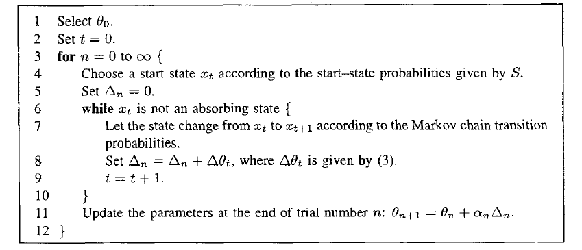
Episodic TD-Lambda algorithm. The parameter vector is updated only at the end of the episode
Daya and Sejnowski (1994) proved parameter convergence with probability 1 under these conditions for TD($\lambda$) applied to absorbing Markov chains in a episodic-setting (i.e., offline).
Bradtke (1994) introduced a normalized version of TD(0) (called NTD(0)) to solve instabilities in the learning algorithm caused by the size of the input vectors $\phi_{x}$
Least-Squares Temporal-Difference Learning
The general problem consists of a system with inputs $\hat \omega_{t} = \omega_{t} + \zeta_{t}$ where $\zeta_{t}$ is the input observation noise at time $t$. For a linear function approximator $\Psi$, we have
\[\begin{align} \psi_{t} &= \Psi(\hat \omega_{t} - \zeta_{t}) + \eta_{t} \nonumber \\ &= \hat \omega_{t}^{\intercal} \theta^{*} - \zeta_{t}^{\intercal} \theta^{*} + \eta_{t} \end{align}\]The quadratic objective function to minimize over all parameter vectors is
\[\begin{equation} J_{t} = \frac{1}{t} \sum_{k=1}^{t} [ \psi_{k} - \omega_{k}^{\intercal} \theta_{t} ]^{2}. \end{equation}\]and the $t^{th}$ estimate of $\theta^{*}$ is
\[\begin{equation} \DeclareMathOperator*{\argmin}{\arg\!\min} \hat \theta^{*}_{t} = \argmin_{\theta_{t}} J_{t} \end{equation}\]We introduce an instrumental variable $\rho_{t}$, which is a vector that is correlated with the true input vectors, $\omega_{t}$, but that is uncorrelated with the observation noise, $\zeta_{t}$. Solving the linear-least squares equation by taking the gradient of the quadratic objective function and setting it to 0 results in this parameter estimate:
\[\begin{equation} \hat \theta^{*}_{t} = \bigg [ \frac{1}{t} \sum_{k=1}^{t} \rho_{k}\hat\omega_{k}^{\intercal} \bigg ]^{-1} \bigg [ \frac{1}{t} \sum_{k=1}^{t} \rho_{k} \psi_{k} \bigg]. \end{equation}\]The correlation matrix $Cor(\rho, \omega)$ must be nonsingular and finite, the correlation matrix $Cor(\rho, \zeta)$ = 0, and the output observation noise $\eta_{t}$ must be uncorrelated with the instrumental variable for $\theta_{t}$ to converge with probability 1 to $\theta^{*}$
We arrive at the LSTD algorithm based on the following assumptions (Lemma 4 in the paper)
- If x and y are states s.t. $P(x,y) \gt 0$
- $\zeta_{xy} = \gamma \sum_{z \in X} P(x,z) \phi_{z} - \gamma \phi_{y}$
- $\eta_{xy} = R(x,y) - \bar r_{x}$
- $\rho_{x} = \phi_{x}$
Then $Cor(\rho, \eta) = 0$ and $Cor(\rho, \zeta) = 0$. In other words, we can use $\phi_{x}$ as the instrumental variable to re-write Equation (5) as:
\[\begin{equation} \hat \theta^{*}_{t} = \big[ \frac{1}{t} \sum_{k=1}^{t} \phi_{k} (\phi_{k} - \gamma \phi_{k+1})^{\intercal}\big]^{-1} \big [ \frac{1}{t} \sum_{k=1}^{t} \phi_{k} r_{k} \big] \end{equation}\]where $\hat\omega_{k} = \phi_{k} - \gamma \phi_{k+1}$ and $\psi_{k} = r_{k}$.
Under some non-too-restrictive conditions, the authors provided proofs of convergence of LSTD on absorbing and ergodic Markov Chains.
Mainly, for absorbing MCs, we need
- The starting probabilities are such that there are no inaccessible states
- $R(x,y) = 0$ whenever $x,y \in T$, the set of absorbing states
- The set of feature vectors {$\phi_{x} | x \in X$} representing non-absorbing states must be linearly independent
- $\phi_{x} = 0$ for all $x \in T$
- Each $\phi_{x}$ is of dimension $N = |X|$
- $0 \leq \gamma \lt 1$
Then $\theta^{*}$ is finite and the LSTD algorithm converges to it with probability 1 as the number of trials (and state transitions) approaches infinity.
There are even less restrictions for convergence on ergodic MCs. The proof of convergence for absorbing MCs is straight-forward.
Convergence of LSTD on absorving Markov Chains
As $t$ grows, the sampled transitions approaches the true transition probability distribution $P$. We also have that each state is visited with probability $\pi_{x}$ (both with probability 1).
Thus, $\theta_{LSTD}$ converges to $\theta^{*}$ with probability 1.
The complexity of LSTD is $O(m^{3})$, where $m$ is the state dimension, since it requires a matrix inversion at every step.
The authors present Recursive LSTD, which is an $O(m^{2})$ version of the LSTD algorithm. It amounts to the TD(0) learning rule, except the scalar step-size parameter is replaced by a gain matrix. See Section 5.4 for the details.
Note that when $rank(\Phi) = n \lt m$, TD($\lambda$), NTD($\lambda$), and RLSTD converge to some $\theta$ depending on the order that states are visited in. LSTD does not converge since the matrix inversion can no longer be computed.
Takeaways
RLSTD (and LSTD algorithms in general) extract more information from each episode. As shown in this paper, even on simple randomly generated Markov Chains, RLSTD produces parameter estimates with significantly lower variance and faster convergence rates than TD($\lambda$) and NTD($\lambda$). Also, the LSTD algorithms don’t have tricky hyperparameters to tune, whereas the TD($\lambda$) algorithms do.
In the experiments in this paper, RLSTD was not sensitive to the initial guess of $\theta_{t}$. It is unclear whether this is always true. On the other hand, TD($\lambda$) is sensitive to the initial guess (obviously, bad guesses = bad performance).
Standard LSTD algorithms require linear function approximators and fixed size feature vectors. These are usually not realistic for high-dimensional spaces and value functions on those spaces. The value function may be nonlinear, and obtaining a feature vector may be difficult or impossible. There is a major need for TD algorithms with nonlinear function approximators and automatic feature extraction that explicitly attempt to keep the variance of the TD-error small.
Some future reading I need to do is on kernel-based LSTD algorithms, that replace the fixed-size feature vector with a kernel.