Part 1: Deploying a PyTorch MobileNetV2 Classifier on the Intel Neural Compute Stick 2
This is the first part of a three part tutorial on using the Intel Neural Compute Stick 2 (NCS2) for vehicle tracking at traffic intersections. The goal of the first part is to get familiar with the NCS2 by walking through how to convert and run a PyTorch MobileNetV2 model on the NCS2 via Windows 10. The following guide should also work for supported popular Linux distros like Ubuntu 18.04.x and 20.04.0 as well as macOS 10.15.x with minor modifications.
Getting started
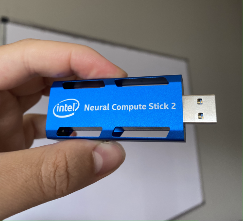
I bought my NCS2 off Amazon for about 80 USD.
We’ll start by setting it up on a Windows 10 PC. My PC has a 6-core Intel i5-9600K processor.
To begin, plug the NCS2 into a USB port on your machine. I then followed the steps from the Intel Windows guide to install their OpenVINO toolkit. As for the dependencies, using Anaconda for Windows to get Python 3.8 was easy and painless. Make sure to follow the steps to install Microsoft Visual Studio 2019 with MSBuild and CMake as well. The only optional step to follow in the guide is to add Python and CMake to your Path by updating the environment variable.
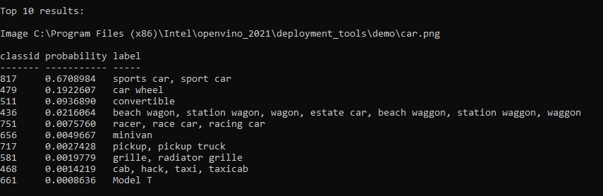
Once you finish, to test the installation, run the following demo in the Windows CLI:
cd "C:\Program Files (x86)\Intel\openvino_2021\deployment_tools\demo"
.\demo_squeezenet_download_convert_run.bat –d MYRIAD
You should see predicted scores:
The PyTorch to ONNX Conversion
Next, we’ll try to port a pre-trained MobileNetV2 PyTorch model to the ONNX format based on this tutorial.
Install PyTorch (cpu-only is fine) following the instructions here and ONNX with pip install onnx onnxruntime. If you are using a clean Python 3.8 conda environment, you may also want to install jupyter at this time.
You can run the code snippets shown throughout the remainder of this guide by downloading and launching this Jupyter notebook. See the ONNX tutorial linked above for detailed explanations of each cell.
# Some standard imports
import numpy as np
import torch
import torch.onnx
import torchvision.models as models
import onnx
import onnxruntime
We can grab a pre-trained MobileNetV2 model from the torchvision model zoo.
model = models.mobilenet_v2(pretrained=True)
model.eval()
Export the model to the ONNX format using torch.onnx.export.
batch_size = 1
# Input to the model
x = torch.randn(batch_size, 3, 224, 224, requires_grad=True)
torch_out = model(x)

# Export the model
torch.onnx.export(model,                     # model being run
                  x,                         # model input (or a tuple for multiple inputs)
                  "mobilenet_v2.onnx",       # where to save the model (can be a file or file-like object)
                  export_params=True,        # store the trained parameter weights inside the model file
                  opset_version=10,          # the ONNX version to export the model to
                  do_constant_folding=True,  # whether to execute constant folding for optimization
                  input_names = ['input'],   # the model's input names
                  output_names = ['output'], # the model's output names
                  dynamic_axes={'input' : {0 : 'batch_size'},    # variable length axes
                                'output' : {0 : 'batch_size'}})
This will create a 14MB file called mobilenet_v2.onnx. Let’s check its validity using the onnx library.
onnx_model = onnx.load("mobilenet_v2.onnx")
onnx.checker.check_model(onnx_model)
Finally, let’s run the model using the ONNX Runtime in an inference session to compare its results with the PyTorch results.
ort_session = onnxruntime.InferenceSession("mobilenet_v2.onnx")

def to_numpy(tensor):
    return tensor.detach().cpu().numpy() if tensor.requires_grad else tensor.cpu().numpy()

# compute ONNX Runtime output prediction
ort_inputs = {ort_session.get_inputs()[0].name: to_numpy(x)}
ort_outs = ort_session.run(None, ort_inputs)

# compare ONNX Runtime and PyTorch results
np.testing.assert_allclose(to_numpy(torch_out), ort_outs[0], rtol=1e-03, atol=1e-05)

print("Exported model has been tested with ONNXRuntime, and the result looks good!")
The ONNX to OpenVINO Conversion
Next we need to pass mobilenet_v2.onnx through the OpenVINO Model Optimizer to convert it into the proper intermediate representation (IR).
I followed the steps listed here.
- Go to
<OPENVINO_INSTALL_DIR>/deployment_tools/model_optimizer. - Run
python mo.py --input_model <PATH_TO_INPUT_MODEL>.onnx --output_dir <OUTPUT_MODEL_DIR> --input_shape (1,3,224,224)
This creates an *.xml file, a *.bin file, and a *.mapping file, which altogether make up the IR for running on the NCS2.
Running the MobileNetV2 IR on the NCS2
Follow along again with the same Jupyter notebook. Download the ImageNet label file and this test image and place them in the same directory as the notebook. In the Windows CLI, run call <OpenVINO_INSTALL_DIR>\bin\setupvars.bat to initialize the Inference Engine Python API, which is needed to import the OpenVINO python libraries (you may need to restart the notebook).
I had to manually edit L38 of <OPENVINO_INSTALL_DIR>\python\python3.8\ngraph\impl\__init__.py to read if (3, 8) > sys.version_info to fix an error. Similarly for L28 of <OPENVINO_INSTALL_DIR>\python\python3.8\openvino\inference_engine\__init__.py. Note that this is seems to be because I am using Python 3.8 and that this may get fixed in a subsequent version of OpenVINO.
from __future__ import print_function
import sys
import os
import cv2
import numpy as np
import logging as log
# These are only available after running setupvars.bat
from openvino.inference_engine import IECore
import ngraph as ng
Then we set some variables and initialize the Inference Engine.
model = "<PATH_TO>\\mobilenet_v2.xml"
device = 'MYRIAD'  # Intel NCS2 device name
log.basicConfig(format="[ %(levelname)s ] %(message)s", level=log.INFO, stream=sys.stdout)
log.info("Loading Inference Engine")
ie = IECore()  # Inference Engine
Read the model in OpenVINO Intermediate Representation (.xml).
log.info(f"Loading network:\n\t{model}")
net = ie.read_network(model=model)
Load the plugin for inference engine and extensions library if specified.
log.info("Device info:")
versions = ie.get_versions(device)
print(f"{' ' * 8}{device}")
print(f"{' ' * 8}MKLDNNPlugin version ......... {versions[device].major}.{versions[device].minor}")
print(f"{' ' * 8}Build ........... {versions[device].build_number}")
Read and preprocess input, following the preprocessing steps for torchvision pre-trained models.
input = 'car.png'
for input_key in net.input_info:
    if len(net.input_info[input_key].input_data.layout) == 4:
        n, c, h, w = net.input_info[input_key].input_data.shape

images = np.ndarray(shape=(n, c, h, w))
images_hw = []
for i in range(n):
    image = cv2.imread(input)
    ih, iw = image.shape[:-1]
    images_hw.append((ih, iw))
    log.info("File was added: ")
    log.info(f"        {input}")
    if (ih, iw) != (h, w):
        log.warning(f"Image {input} is resized from {image.shape[:-1]} to {(h, w)}")
        image = cv2.resize(image, (w, h))
    # BGR to RGB
    image = cv2.cvtColor(image, cv2.COLOR_BGR2RGB)
    # Change data layout from HWC to CHW
    image = image.transpose((2, 0, 1))
    # Change to (0,1)
    image = image / 255.
    # Subtract mean
    image -= np.array([0.485, 0.456, 0.406]).reshape(3,1,1)
    # Divide by std
    image /= np.array([0.229, 0.224, 0.225]).reshape(3,1,1)
    images[i] = image
Prepare input and output data. We use the default FP32 precision, but for future use, we could explore models that use lower precisions for faster runtimes.
log.info("Preparing input blobs")
assert (len(net.input_info.keys()) == 1 or len(
    net.input_info.keys()) == 2), "Sample supports topologies only with 1 or 2 inputs"
out_blob = next(iter(net.outputs))
# Just a single output, the class prediction
for input_key in net.input_info:
    input_name = input_key
    net.input_info[input_key].precision = 'FP32'
    break

data = {}
data[input_name] = images
Load the model to the NCS2 and do a single forward pass.
log.info("Loading model to the device")
exec_net = ie.load_network(network=net, device_name=device)
log.info("Creating infer request and starting inference")
res = exec_net.infer(inputs=data)
Display the top 10 predictions.
log.info("Processing output blob")
log.info(f"Top 10 results: ")
labels_map = []
with open('mobilenet_v2.labels', 'r') as f:
    for line in f:
        labels_map += [line.strip('\n')]
classid_str = "label"
probability_str = "probability"
for i, probs in enumerate(res[out_blob]):
    probs = np.squeeze(probs)
    top_ind = np.argsort(probs)[-10:][::-1]
    print(f"Image {input}\n")
    print(classid_str, probability_str)
    print(f"{'-' * len(classid_str)} {'-' * len(probability_str)}")
    for id in top_ind:
        det_label = labels_map[id] if labels_map else f"{id}"
        label_length = len(det_label)
        space_num_before = (7 - label_length) // 2
        space_num_after = 7 - (space_num_before + label_length) + 2
        print(f"{det_label} ... {probs[id]:.7f} %")
    print("\n")
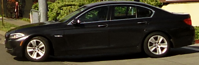
car.png
Result:
label probability
----- -----------
convertible ... 11.8281250 %
beach wagon, station wagon, wagon, estate car, beach waggon, station waggon, waggon ... 11.5546875 %
sports car, sport car ... 11.4296875 %
pickup, pickup truck ... 11.2734375 %
car wheel ... 10.7968750 %
grille, radiator grille ... 10.3515625 %
Model T ... 8.8203125 %
minivan ... 8.7578125 %
cab, hack, taxi, taxicab ... 8.5625000 %
racer, race car, racing car ... 8.1250000 %
Great! In part two of this tutorial, we’ll step through the process of running MobileNetV2-SSDLite for object detection on the NCS2 with a Raspberry Pi.
References
- Sandler, Mark, Andrew Howard, Menglong Zhu, Andrey Zhmoginov, and Liang-Chieh Chen. “Mobilenetv2: Inverted residuals and linear bottlenecks.” In Proceedings of the IEEE conference on computer vision and pattern recognition, pp. 4510-4520. 2018.